Surrogate models for model-in-the-loop control

Introduction

Numerical simulations play a crucial role in the design, analysis, and control of mechanical systems. Finite element (FE) models are frequently used because they can accurately describe complex physical phenomena. However, this often comes with high computational costs, making extensive parameter studies, interactive use, or the use of the model in online control (model-in-the-loop) unfeasible.

To overcome these limitations, surrogate models are increasingly being used. These are simplified, data-driven machine learning models that can approximate the results of a complex model, but with significantly lower computation times.

In this article, we will guide you through the process of creating such a surrogate model for an FE model that calculates the forces on a conveyor belt.

The Conveyor Belt Model

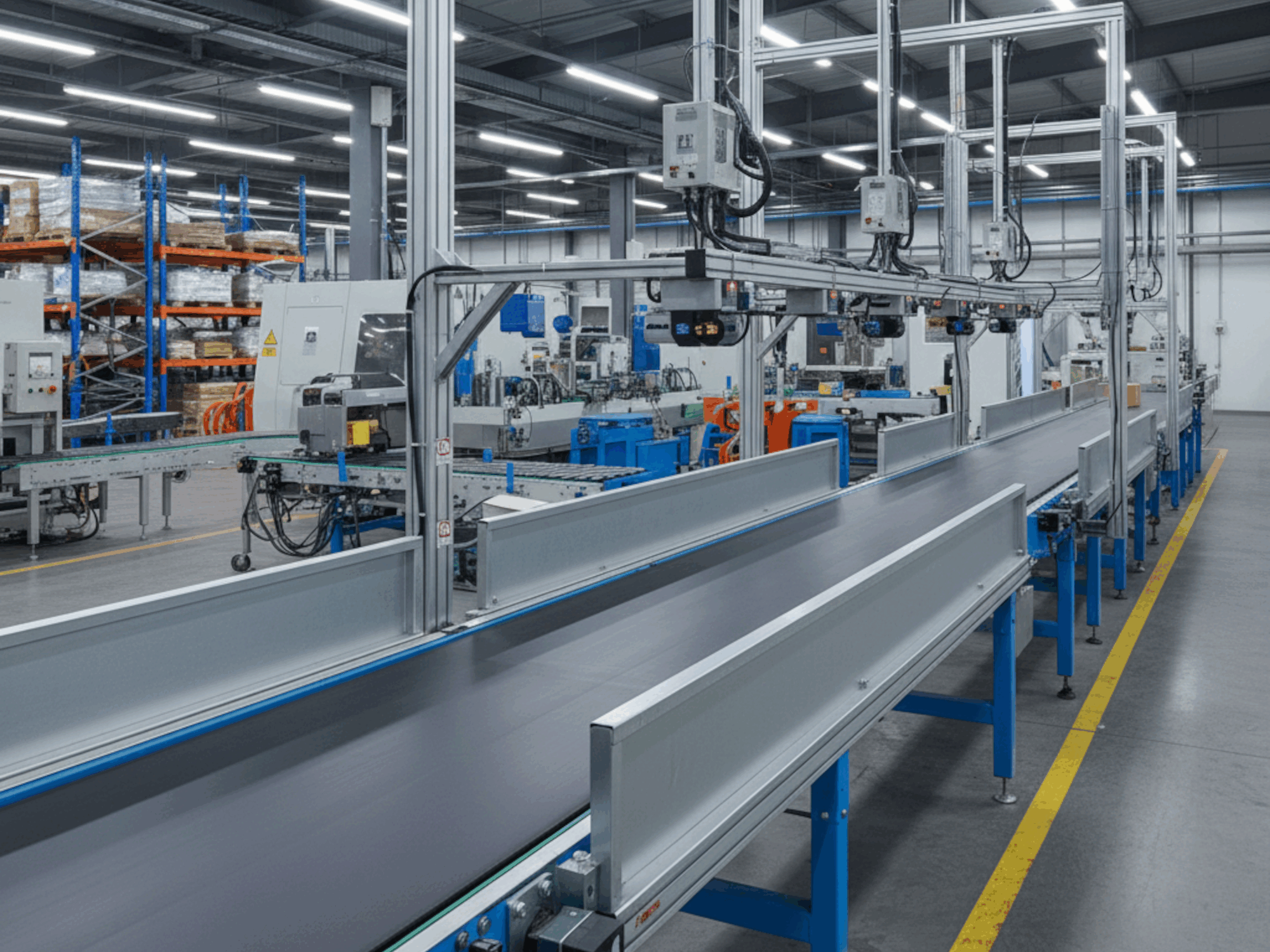
Conveyor belts are used in many equipment and industrial applications. Belt systems generally have a drive roller, one or more tracking rollers, sometimes one or more tension rollers, and a few rollers to form the desired path for the belt.

In the FE model we will be using, the forces and displacements on the belt are calculated on a grid. The model has a typical number of grid cells for such a belt system calculation. The relative positioning of the belt along the entire path is particularly important for our application.

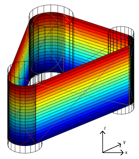
The system consists of three rollers: a drive roller, a tracking roller that can tilt in two directions, and a third roller to form the belt path. The input variables of the belt tracking model are the angles of the tracking roller in the x and y directions, and the rotational speed of the drive roller. The output is a grid with values ​​for the lateral (z direction, in Figure 1) deviation in position. This deviation provides us with the information about the belt deformation we need to properly adjust the system.

Because understanding the model is not important for the data-driven surrogate model, but only for approximating the output data, we do not need to know any further details about the equations solved by the FE model.

Data-Driven Model

Data Generation & Model Reduction

A first step in creating a data-driven surrogate model is generating a large amount of data. We performed hundreds of calculations for various combinations of input parameters, always reaching a steady state—the converged state that no longer changes over time, which occurs when the simulation is run long enough.

To reduce the size of the surrogate model, we used a reduced order model based on singular value decomposition; the model then predicts only the values ​​for the most important modes. We calculated the most important modes that occur in the resulting lateral deviations from the steady states. The first modes are shown in Figure 2, where the tire has been cut and laid flat to create the plots. The first mode is hard coded to the offset mode: a single constant value for each grid cell on the tire. Each pattern represents a dominant deformation mode of the tire.

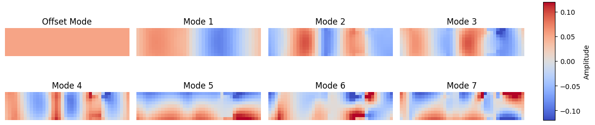
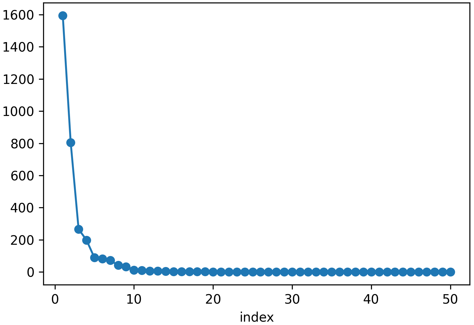
Figure 3 shows the scree plot of the singular values. The sharp decline indicates that the first eight modes already explain most of the variation. This justifies our choice to predict only these coefficients with the surrogate model.

Together, these eight modes form a compact but expressive representation of the physics. The surrogate model therefore does not need to reconstruct the complete band behavior but only estimates these eight coefficients—a huge gain in computational time.

The neural network

The surrogate model takes the three simulation parameters (the angles of the steering roller in the x and y directions, and the rotational speed of the drive roller) as input and predicts eight coefficients for the solution in terms of the eight modes.

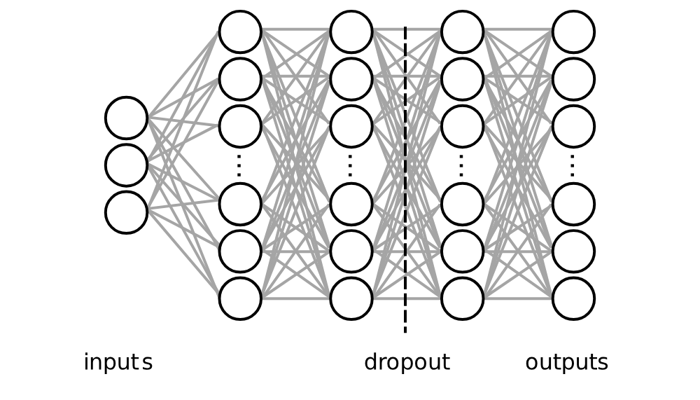
We use a simple neural network with three fully connected hidden layers and a dropout layer to prevent overfitting—a total of 1,289 free parameters for training. The loss function is the mean squared error over the reduced basis coefficients.

The neural network was created using the Tensorflow library for Python. The results are logged using MLflow—this allowed us to easily experiment with different network architectures. After aggregating and comparing the different network architectures, the best architecture was selected.

Results

After training the neural network, the model’s accuracy is tested on a test dataset. Figure 5 shows some predictions from the neural network.

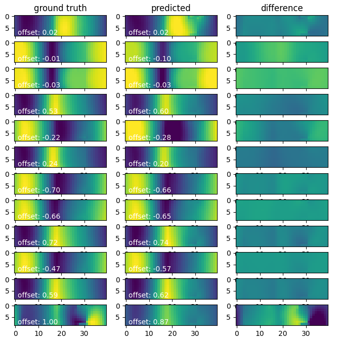
A good, practically useful measure of the error is the Root Mean Squared Error (RMSE) – the square root of the sum of the squares of the error at each coordinate. We then take the RMSE over the last seven coefficients of the reduced order basis, and not over the offset. The offset is less important in our application – the focus is on the relative deformation of the tire. The median of this RMSE across all test data samples is half a millimeter, on a 320-millimeter-wide tire.

As can be seen from the difference in colour pattern in the last state in Figure 5, the neural network has difficulty predicting extreme cases. In this example, the tire falls off a roller. There are only two cases of this in the entire dataset, so the surrogate model cannot handle them well.

Conclusions & Discussion

In most cases, the surrogate model is a good approximation of the full model. It makes a prediction in a fraction of a second, while the original FE model needed ten minutes. In situations where many cases need to be calculated quickly, for example, during system design or real-time control, such a surrogate model could be very useful.

This case study was merely a proof of concept; many improvements are still possible for this model. First, more extreme cases could be added to the dataset so that the surrogate model can also accurately predict these cases. We could also incorporate more physics knowledge into the loss function. Furthermore, we could create a model that predicts a single time step of the FE model, instead of the steady state. This would then allow us to model the time-dependent behavior as well.

An ML surrogate for your computing model

Do you also work with demanding calculation models, and could a fast, data-driven surrogate model be a useful addition to your workflows? Then contact VORtech! Our data scientists are good at understanding the scientific context of calculation models and can translate customer requirements into solid software solutions that use modern machine learning.

You can find more information about our approach to machine learning here. If you want to follow what we’re doing in this field, our newsletter may be a good option for you, or else our LinkedIn page.

Meer informatie over onze benadering van machine learning kunt u hier vinden. Als u wilt volgen wat wij op dit gebied doen, is onze nieuwsbrief een goede optie, evenals onze LinkedIn-pagina.