
Experiments with simple model-order reduction methods
The time needed to run a model is often an issue in things like design optimization, model-based predictive control, or digital twinning. In many cases, this issue can be solved by using an approximate model that is less accurate but much faster. In this blog, we’ll give a very basic introduction to these techniques and describe some experiments that were done at VORtech by two interns at VORtech, Floris Roodenburg and Abinash Mishra. They could speed up calculations for several industrial problems by more than a factor of ten.
Model-order reduction is a powerful technique to speed up simulations. It can be used to solve performance issues in applications like design optimization, model-based predictive control, or digital twinning. In this blog, we’ll give a very basic introduction to these techniques and describe some experiments that were done at VORtech by two interns at VORtech, Floris Roodenburg and Abinash Mishra. They could speed up calculations by more than a factor of ten.
The term that is used for constructing approximate models is Model-Order Reduction or Reduced-Order Modelling. The two terms are mostly used interchangeably, but for this article, we will use the first as it implies that we start with a model and then reduce it. The term Reduced-Order Modelling might suggest that you build a model of reduced order in the first place. That is not what we are doing here.
Another term that is also used in this context is surrogate models, which somewhat widens the category because it suggests that the model can be replaced by something that is not closely related to the full model. Still, surrogate models are also often made from data that is generated by a full, detailed model.
When (not) to use Model-Order Reduction
Model-Order Reduction throws away some of the details in the model. So, it should only be used if those details are not that important. You would not use it, for example, for model-based predictive control of a highly sensitive process.
There are many cases where a model does not need to be very accurate. For example, when you are designing a product and you want to run an optimization algorithm to find the best parameters for the design, you don’t need all the details in the early phases of the optimization. As long as the algorithm just gets the general direction ok, you’re fine. The details will only matter when you approach the optimum but at that point, you usually have done most of the optimization iterations already.
Another example where a simplified model is extremely useful is data assimilation. Here, you use data to estimate the parameters or state of your model. By running an optimization algorithm, the parameters are found that give the best match between the data and the model. Again, you do not need all the details early on in this process. In some cases, you do not need them at all if you just want your model parameters to be good enough rather than perfect.
Similarly, when you are doing model-based predictive control of a well-behaved and non-sensitive or non-critical process you are just aiming for a good-enough solution, and you could well do without the accuracy of a full model.

The broad picture
There are many ways to approximate a model. The wonderful series of Open Access books on the subject are testament to that. Here, we will only give a very elementary outline.
Broadly speaking, model-order reduction methods can be divided into intrusive and non-intrusive approaches.
Intrusive methods are the most elegant in terms of the underlying mathematics. They largely respect the physics that is in the model. However, this method is not easy to apply as you need to change the model code considerably. Developing an intrusive reduced-order model can take months if not years in case of complex models.
Non-intrusive methods are far easier to use; they can typically be developed in the order of a few weeks or less. They treat the model as a black box and are thus ideally suitable in situations where you do not have access to the model code or if you do not want to change that code. In fact, you do not need the model but only the result of the model runs of the full model for various settings of parameters and input. These results are enough to construct the approximate model. In that sense, most non-intrusive methods are essentially data-driven methods.
The drawback of non-intrusive methods is that the reduced-order model has no understanding of the physics in the model. It needs to make do with the data that it gets. Therefore, such an approximate model is typically only valid for model parameters that are close enough to the parameters that were used to build the approximate model. Because of its lack of understanding of the physics, the reduced model simply cannot know what goes on beyond the approximation region.
These days, it is also becoming fashionable to use for example neural networks as an approximate model. This is an obvious idea as neural networks are, in a way, just hugely sophisticated function approximations that could learn the transfer function between parameters and history on one side and model results on the other side. We will not go into this approach in this article as we did not try it yet.
An example use-case
Floris Roodenburg, an exceptionally good MSc student from the Mathematics Department of Delft University of Technology did an internship at VORtech to experiment with a few non-intrusive methods. We wanted to get a general feeling for the pros and cons of the various methods and to understand the applicability and limitations of model-order reduction in general. Thea Kik-Vuik from VORtech was the supervisor for this internship.
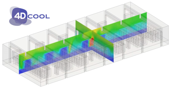
As a case study, we used the 4DCOOL project, which is a digital twin of the climate in server rooms in datacenters. 4DCOOL helps operators in data centers to use the cooling equipment more efficiently. The idea is that this will save costs and lead to a lower carbon footprint, which are both relevant KPIs for data centers.
Operators use 4DCOOL to visualize the current temperature and flow in the server room and, if they see an opportunity for improvement, run simulations to explore the options.
At the core of 4DCOOL is a CFD-model based on OpenFOAM. The parameters of the model are constantly tuned to match the model with the latest values from the temperature sensors in the server room. Right now, the most important parameters for 4DCOOL are the heat loads from the servers. These are unknown and therefore have to be estimated from the measured temperatures.
This tuning of parameters is done with a data-assimilation method, which is essentially an optimization method to optimize the values of the parameters for the given observed temperatures. The optimization requires a significant number of model runs. Depending on the complexity of the server room, the full model can take up to an hour to compute. This is unfeasible considering the continuous updating of the parameters. But the parameter estimation doesn’t really need all the accuracy of the full model. Therefore, 4DCOOL is a wonderful candidate for model-order reduction.
We were lucky to get a lot of support from Professor Arnold Heemink, who has extensive expertise in the technologies that are involved here; from Actiflow, a company that specializes in CFD and from Kelbij Star and Giovanni Stabile, who are working on intrusive Model-Order Reduction methods for OpenFOAM. Kudos to them.
A very simple model-order reduction for 4DCOOL
As stated above, an intrusive method would be the most elegant. In fact, an effort is already underway to implement model-order reduction in OpenFOAM. But at the time of the internship, this effort, called ITHACA-FV, still lacked some features that we needed for our purposes. This again highlights the fact that implementing an intrusive method is far from easy.
A non-intrusive method was more feasible. For us, an additional benefit was that experience with these methods was even more valuable as our clients will often not have the budget to go all-out on model-order reduction. At least not until its value has been demonstrated. Thus, they are likely to start experimenting with non-intrusive methods and might look to us for support.
One of the various methods that Floris explored was Proper Orthogonal Decomposition with Interpolation (PODI). There is a nice open-source Python library available for this, called EZyRB. For mathematicians: the basic idea is to run the original model for a range of parameter settings and time instances, collect the result vectors (“snapshots”) in a matrix and make a Singular-Value Decomposition of that matrix. This provides you with the most important patterns (modes) of the result space . The reduced space is now spanned by these most important modes. Computing a solution for a given set of parameters is then a simple interpolation between the appropriate snapshots. This is then followed by a simple back-transform from the reduced model space to the full model space. For the interpolation between snapshots, you can use simple linear interpolation or be a bit more sophisticated with radial basis functions.
Obviously, with PODI you first have to construct the snapshots, which means running the model for a sufficient sampling of the parameter space. We used a very coarse sampling: only four potential values for the heat loads of each of four servers but this already amounts to 256 snapshots for a single time instance. With ten snapshots, one for each of ten minutes, the total amount of snapshots is 2.560. In our case, it took some eight hours to compute all the 2.560 snapshots.
But this is done entirely offline before the operational phase of the model. Once the snapshots are computed, the rest is really fast. Building the reduced model from the snapshots takes only around 8 seconds and a single evaluation of the reduced model took less than 1.5 seconds. This is far less than a run of the full model for ten timesteps, which takes around 2 minutes. This is not too surprising as we are in fact doing just an interpolation and a back transformation. Also, the interpolation is done on a much smaller state space than the original model. Whereas the original model had a size of some 8.000 grid points, the reduced model needed only some 5 to 10 modes.
The bad news is that the errors tended to be rather large at specific points in the server room. Even though the average error was somewhat acceptable at around 1 degree Celsius, it could go up to 16 degrees close to the servers, which is exactly the location where it matters most. The main culprit was, however, not the model-order reduction as such but the interpolation between snapshots.

Estimating parameters with a Reduced-Order Model
Even though the errors in the reduced model were significant, we were interested to see how serious it would be when we would use the reduced model for parameter estimation. Perhaps we could use the reduced-order model to get close to the right parameters and then do the last refinement of the parameters quickly in the full model space.
We were lucky to find yet another enthusiastic intern in Abinash Mishra, a student from the Applied Sciences Faculty of the Delft University of Technology. He built a framework for finding the parameters in a simulation using a reduced-order model for which he used the research and support of Arnold Heemink. The basic idea is to construct a small, linear model from snapshots of the full nonlinear model. As the small model is linear, it can be efficiently used to find the model parameters that make for the best match between the model and the observations.
Because the full model is nonlinear, the parameters that are found may not be entirely correct if they are too far from the ones for which the linearization was made. Therefore, a new linearization may be needed around the parameters that were found. This may repeat itself a couple of times to eventually find the optimal parameters for the non-linear full model. If enough of the parameter search can be done in reduced space and if building the linearization is not too expensive, then this approach can save a lot of time.
Abinash demonstrated his software on a rather simple heat-diffusion problem on a square domain. This is actually a linear model so that the linearization was trivial. We deliberately used this simple example because it would allow us to fully understand all the intermediate results in the computation.
The results were rather spectacular. Where the parameter search with the full model (state space of dimension 2500) needed 240 seconds, the version with a reduced model (4 modes out of 200 snapshots) took only 6 seconds. That is a speedup of a factor of 40. Note, however, that this is a linear model, and a re-linearization is not needed in this case. A non-linear model will probably have less speedup. However, this was only a very first experiment and further optimizations are conceivable. In the literature, similar speedups are not uncommon. The result was also accurate: the estimated parameter value (in this case the heat source) had an error of only 0.002%. Again: this is at least partly due to the very simple nature of the model.
All this does not tell us much about the use for the 4DCOOL model. The example heat-diffusion model that was used for the experiments is very regular and behaves nicely whereas the 4DCOOL models have a very complex topology and complex physics. But at least we now have working software in which we can start experimenting with the actual challenge at hand. We hope to find another intern soon to make this next step.
Is Model-Order Reduction interesting for your application?
If all of this could be interesting for your application, feel free to reach out to us. We would be happy to share our experiences and insights with you. If you are planning to implement methods like these to speed up your application, our scientific software developers are here to help you.